A diversion into hydrogen states.
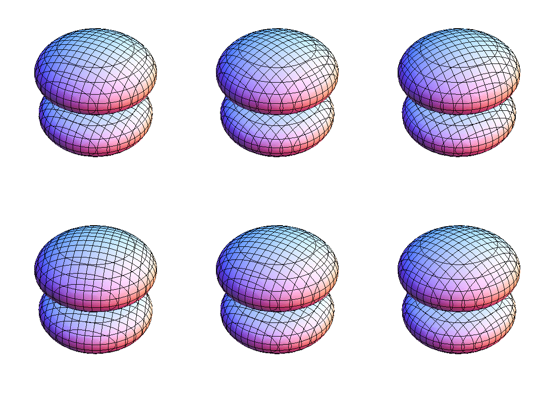
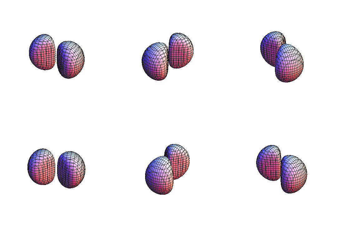
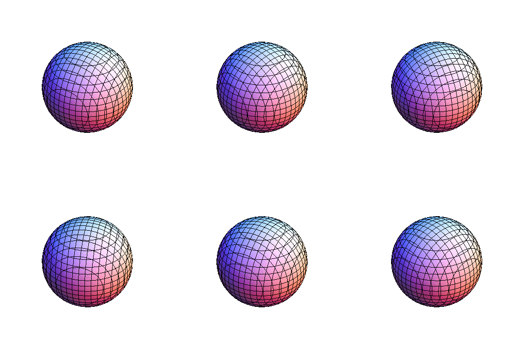
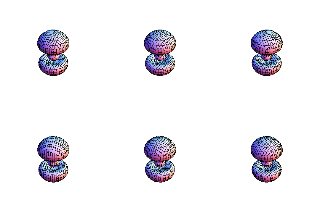
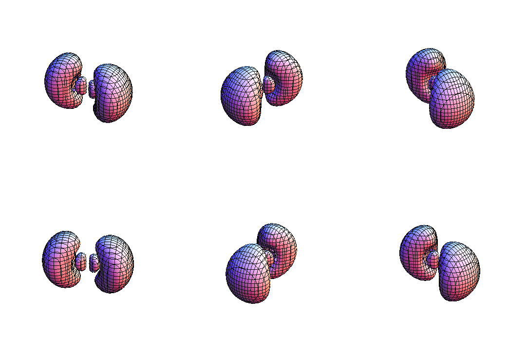
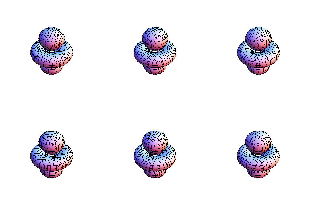
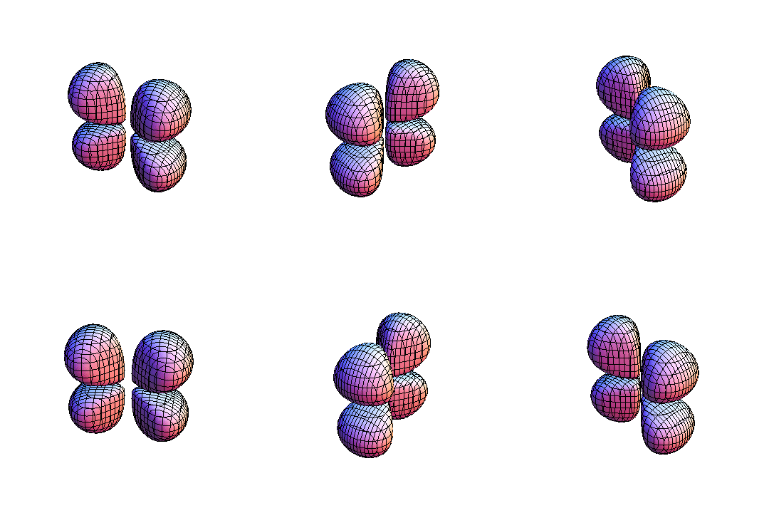
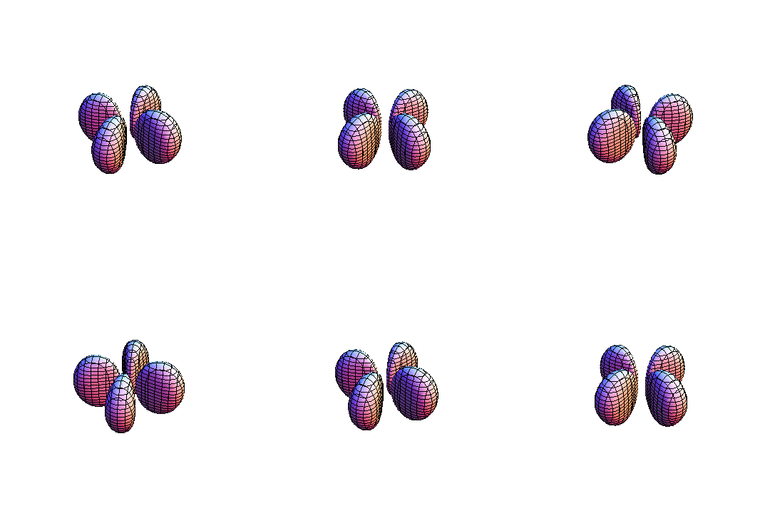
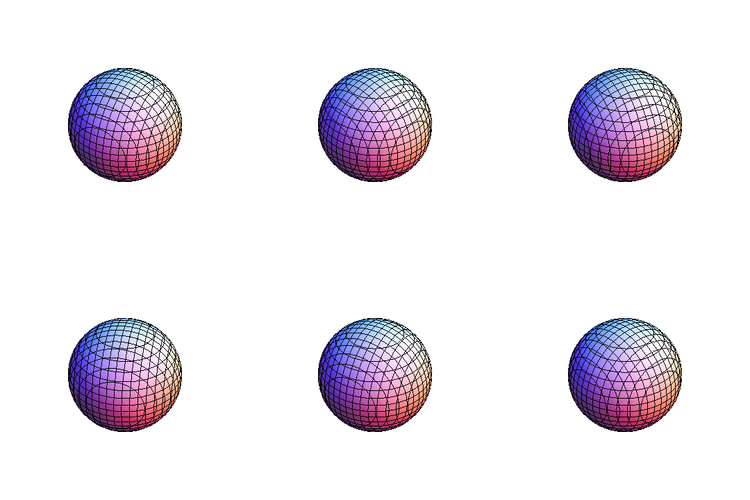
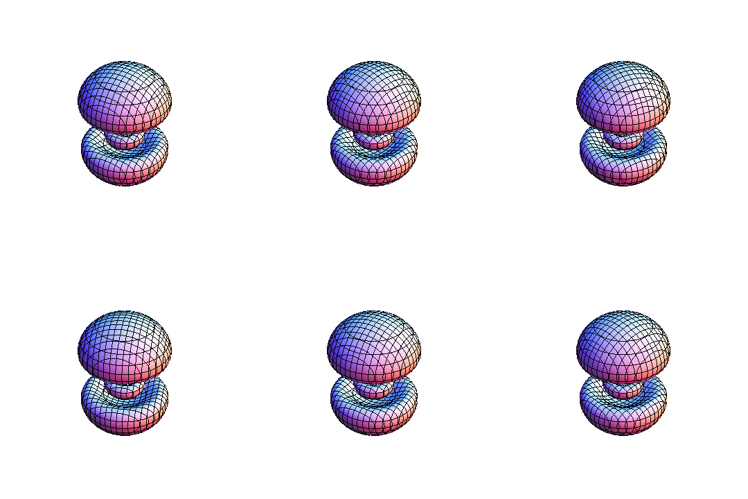
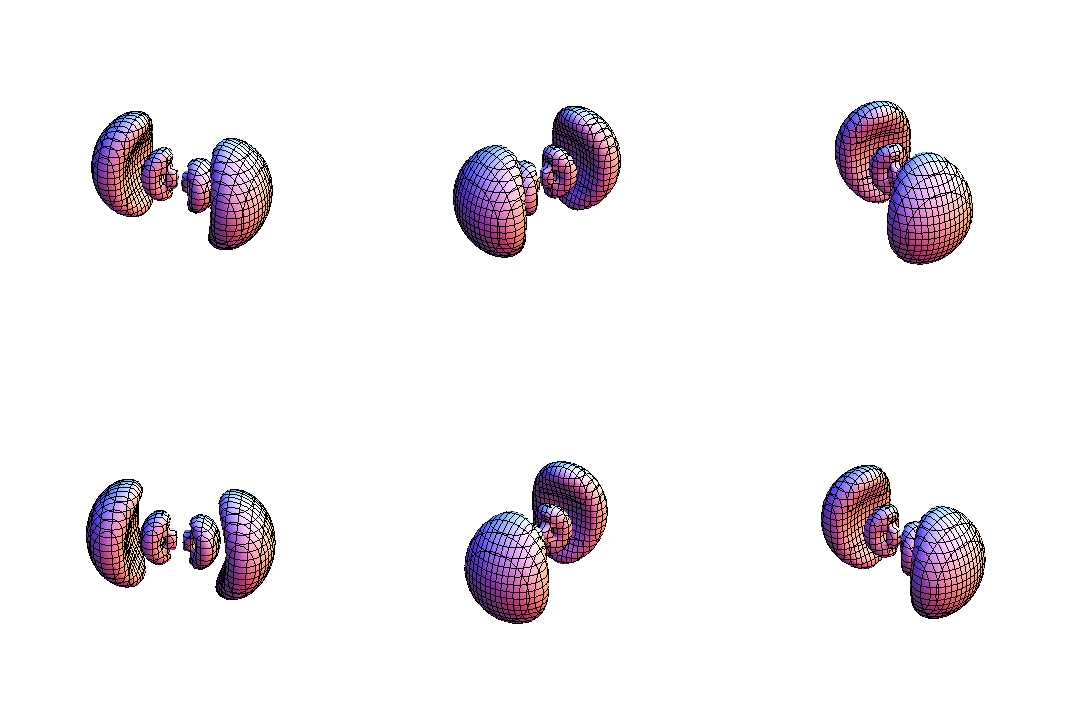
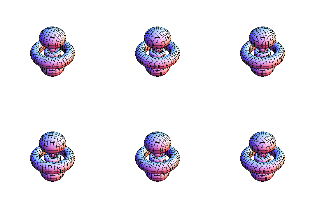
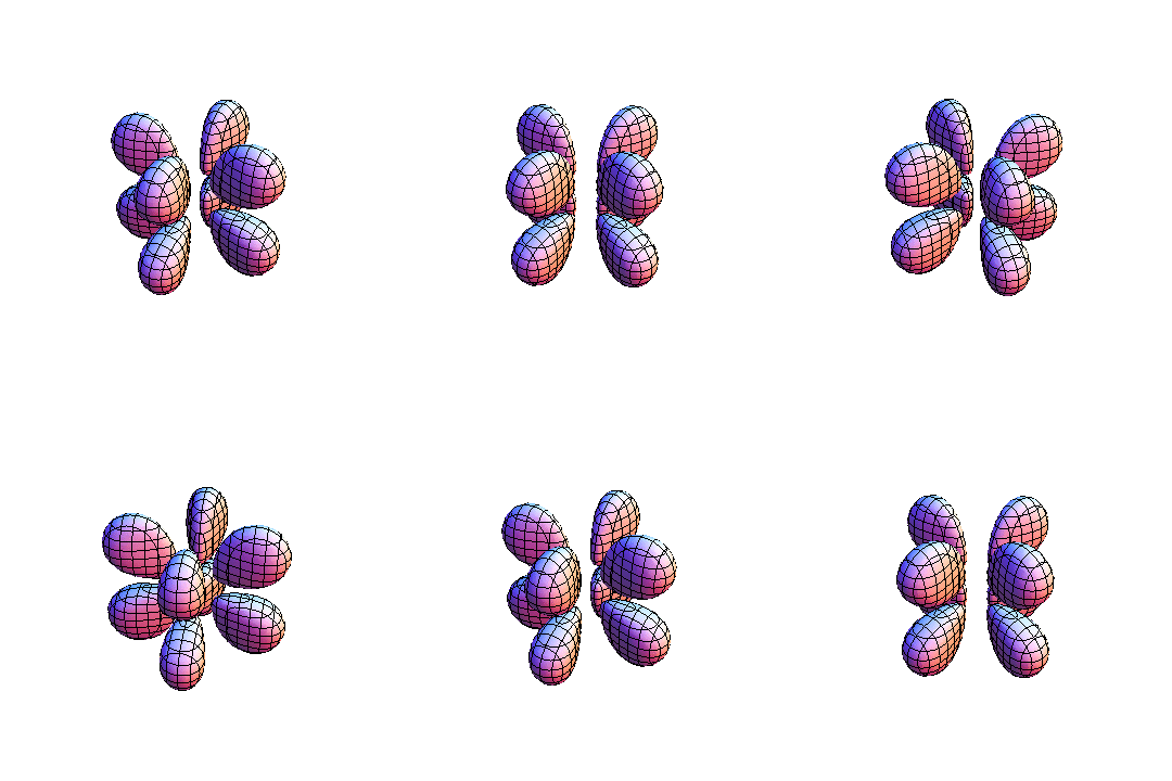
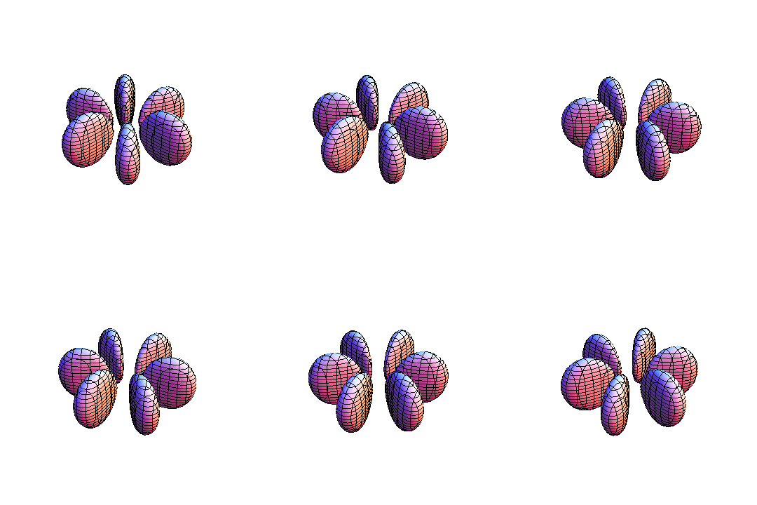
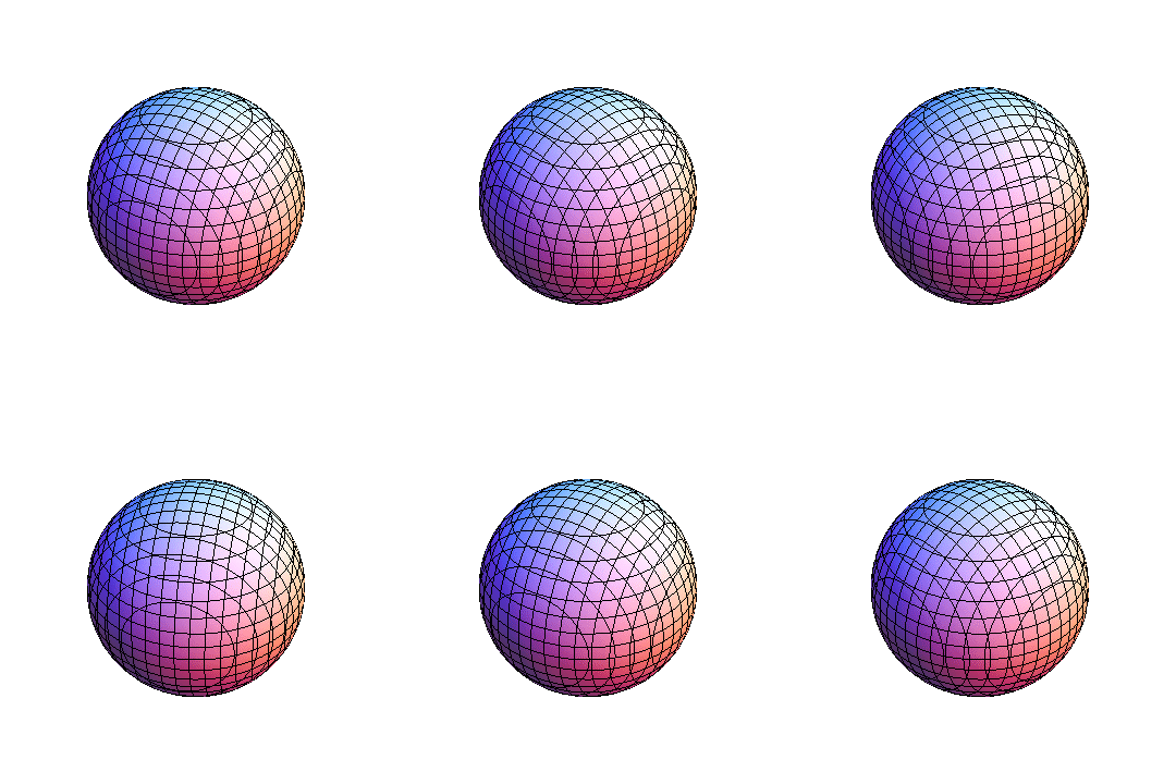
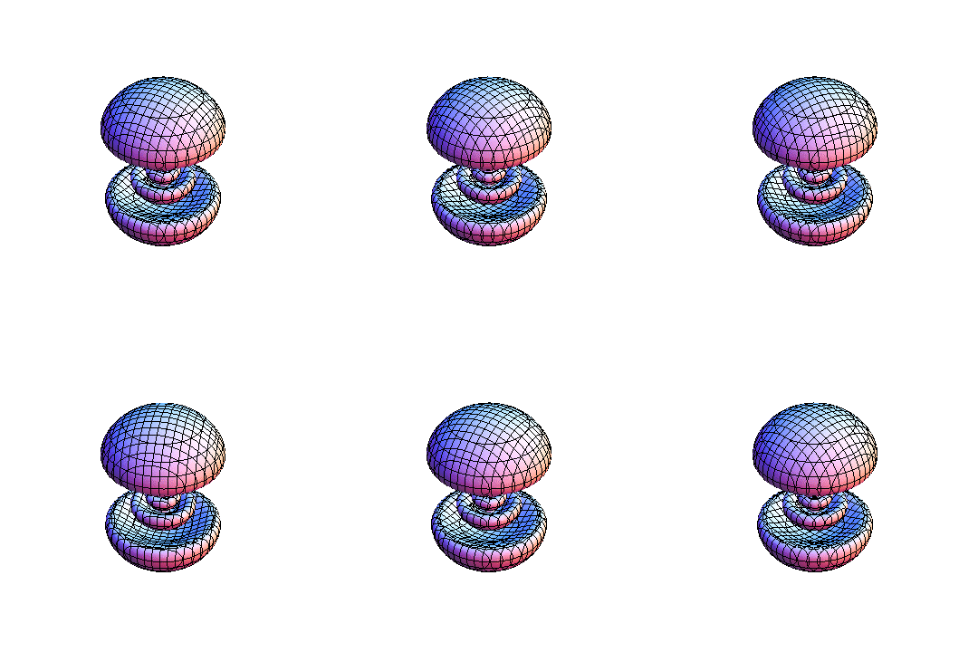
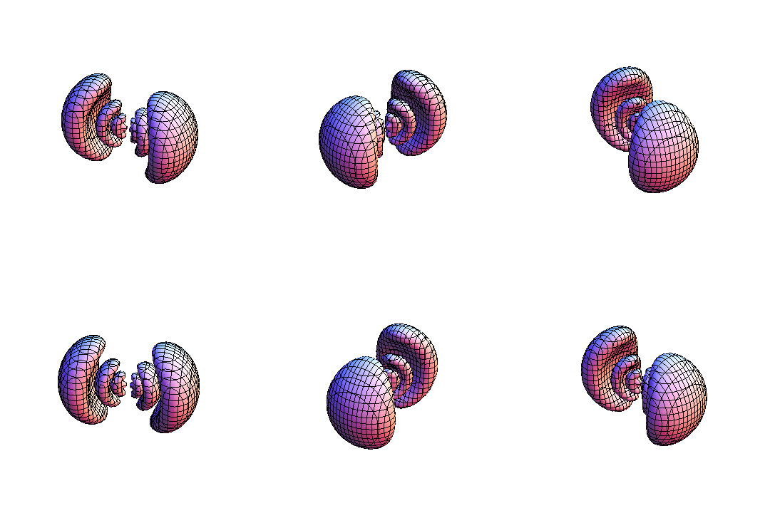
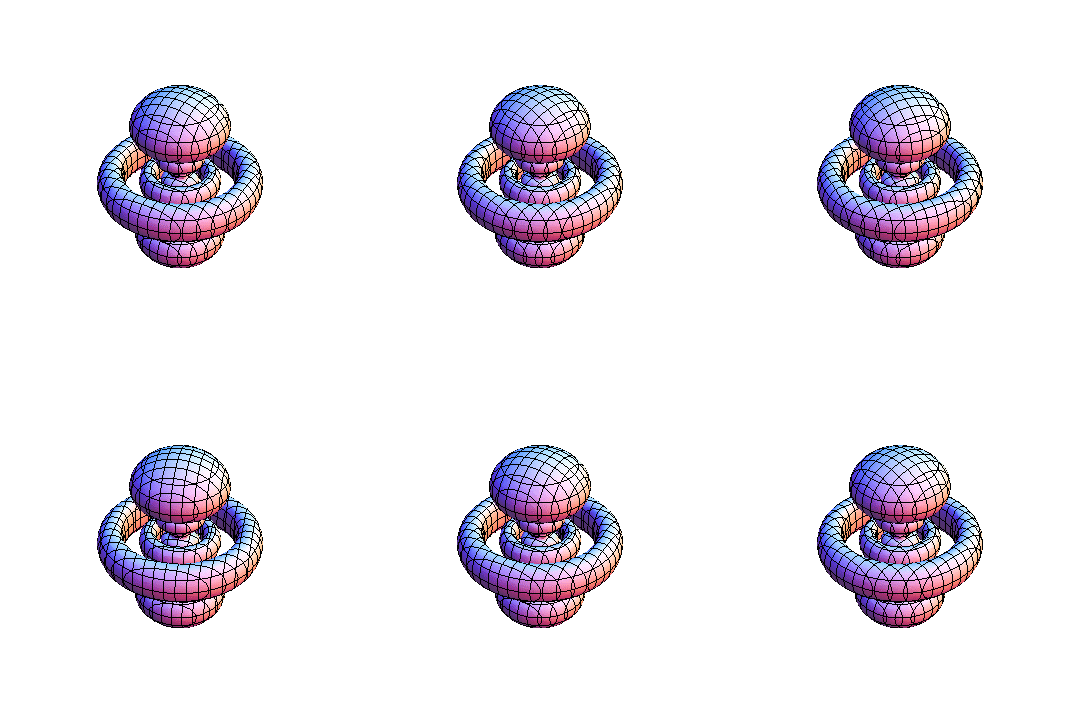
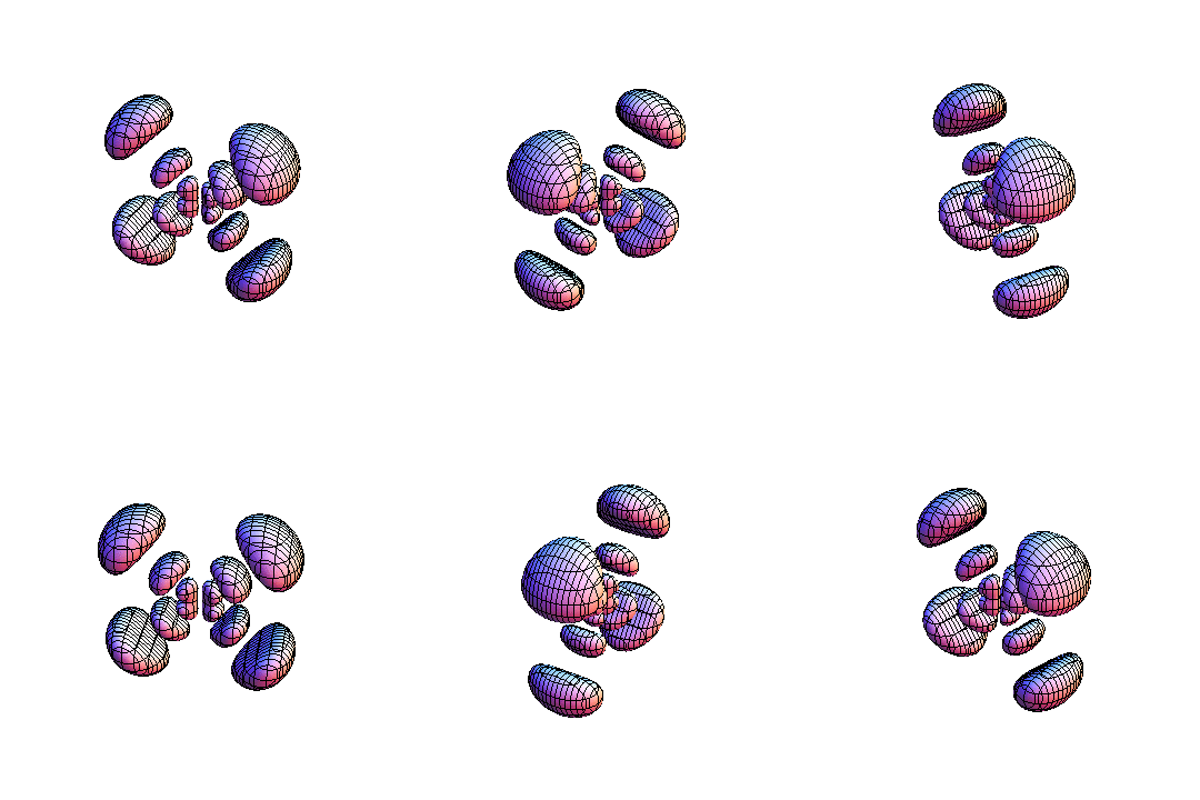
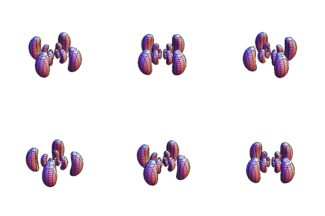
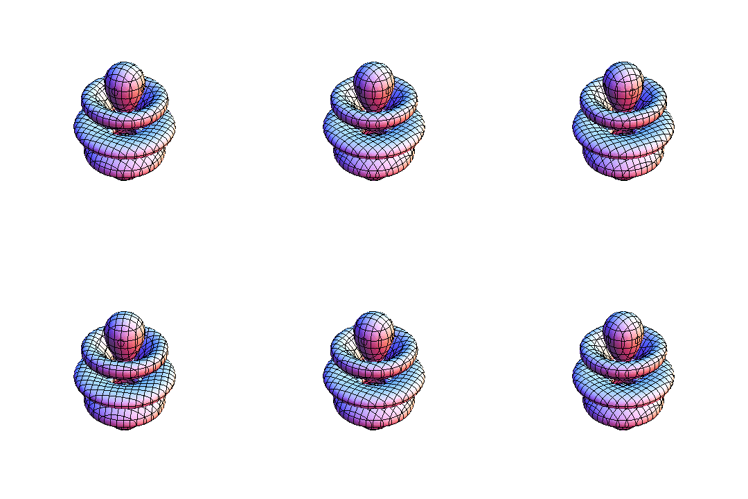
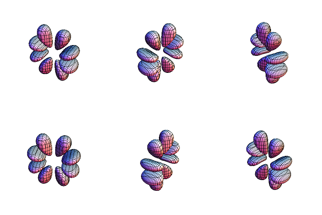
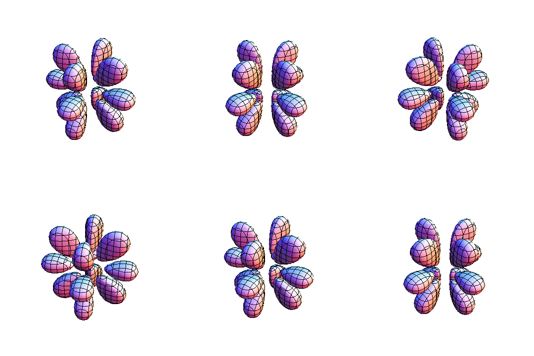
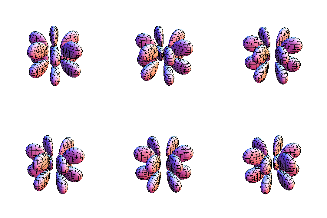
I made an animated table of hydrogen-state visualizations in Mathematica while putting off a writing assignment. All 35 states from the original collection are here: n = 1 through n = 5, with 0 ≤ l < n and 0 ≤ m ≤ l.
A note on interpretation. These are historical visualization experiments. The original page describes plotting Re(ψ²), which is different from the probability density |ψ|². These shapes should not be read as faithful probability-density plots, and their displayed sizes are not to a common scale.
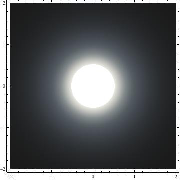
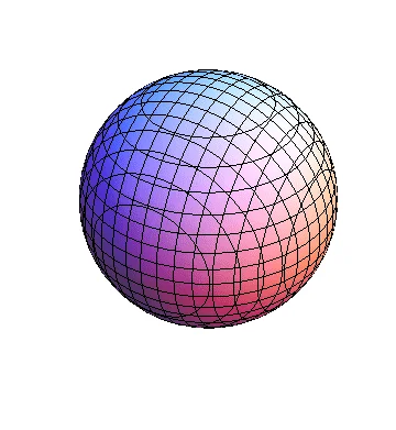
Open the original animations
n = 1
1s, m=0
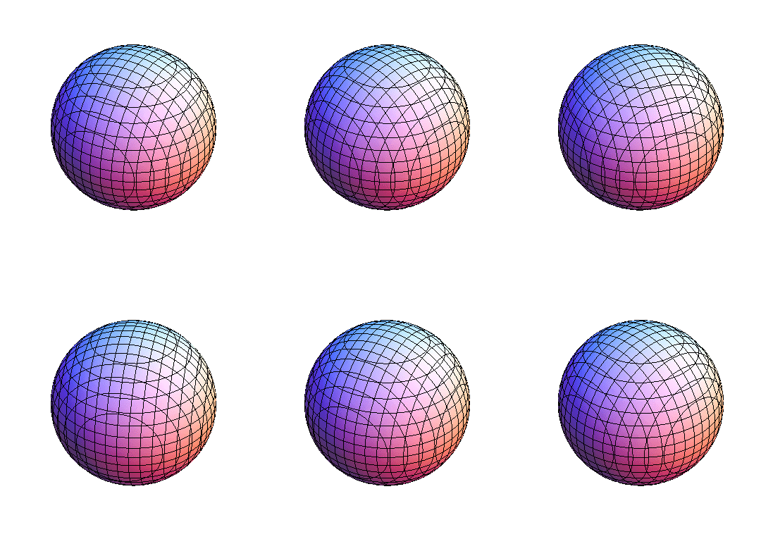
n = 2
2s, m=0 ·
2p, m=0 ·
2p, m=1
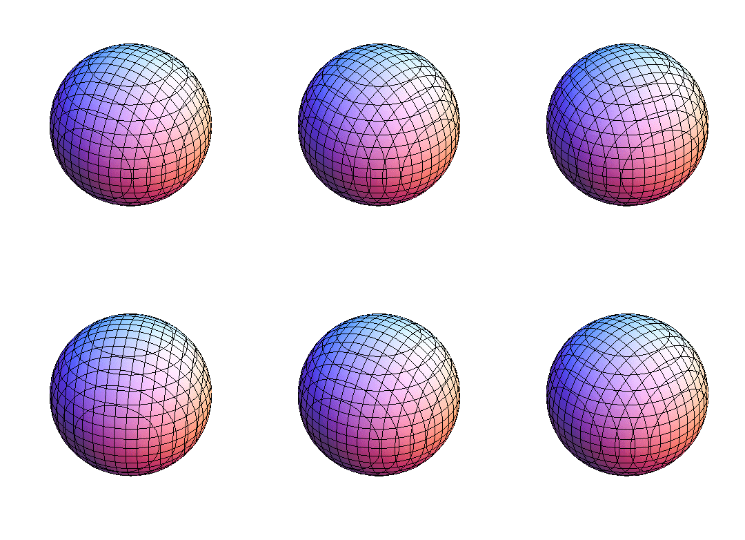
n = 3
3s, m=0 ·
3p, m=0 ·
3p, m=1 ·
3d, m=0 ·
3d, m=1 ·
3d, m=2
n = 4
4s, m=0 ·
4p, m=0 ·
4p, m=1 ·
4d, m=0 ·
4d, m=1 ·
4d, m=2 ·
4f, m=0 ·
4f, m=1 ·
4f, m=2 ·
4f, m=3
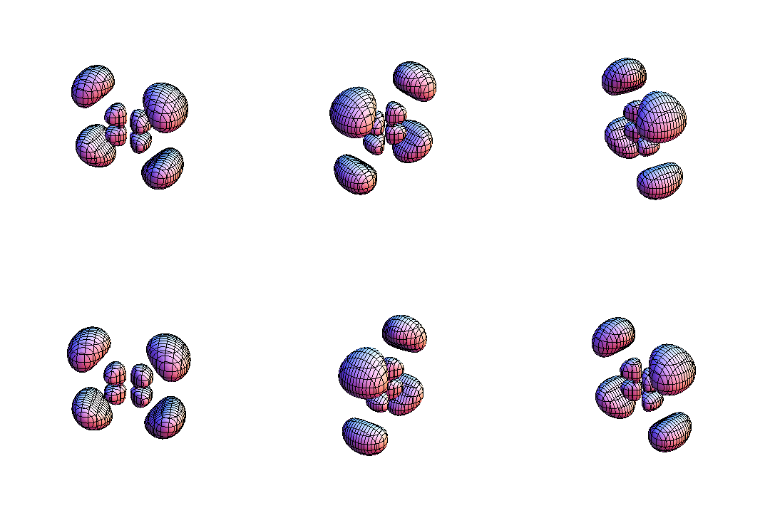
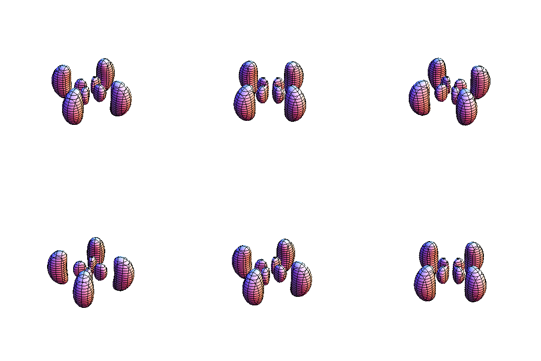
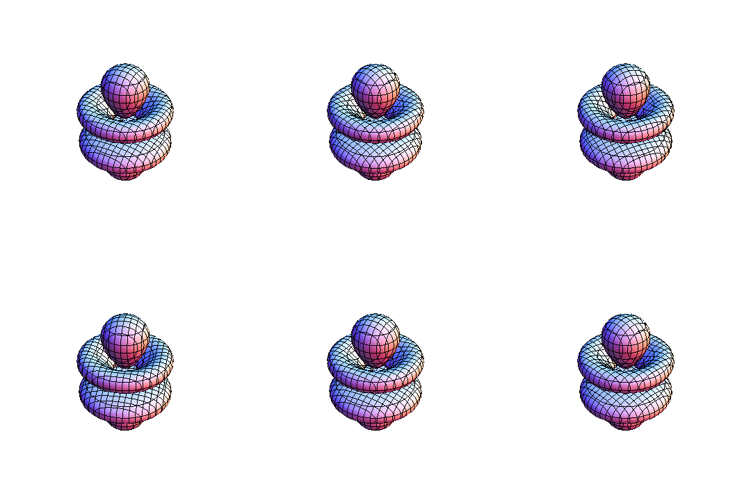
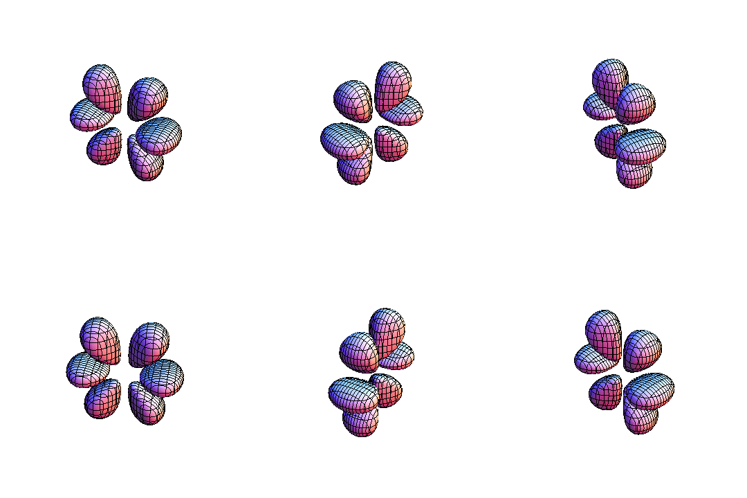
n = 5
5s, m=0 ·
5p, m=0 ·
5p, m=1 ·
5d, m=0 ·
5d, m=1 ·
5d, m=2 ·
5f, m=0 ·
5f, m=1 ·
5f, m=2 ·
5f, m=3 ·
5g, m=0 ·
5g, m=1 ·
5g, m=2 ·
5g, m=3 ·
5g, m=4
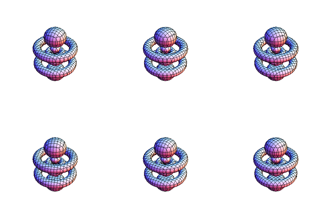
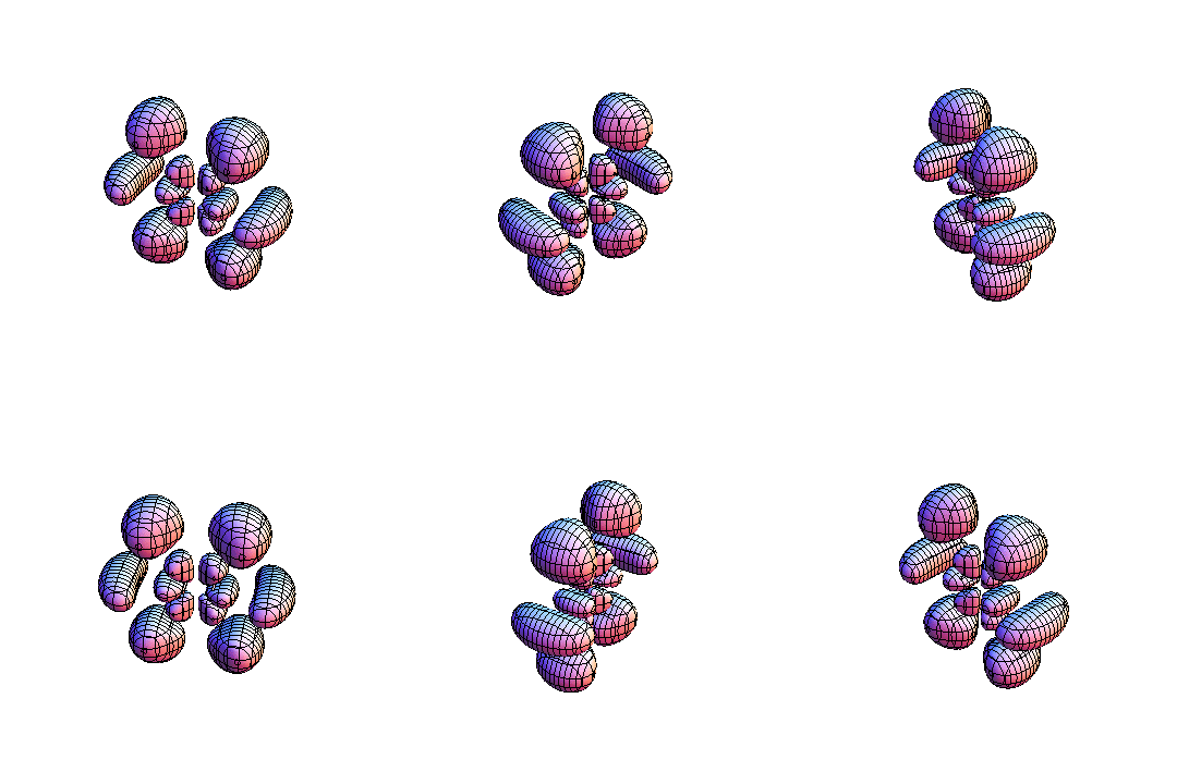
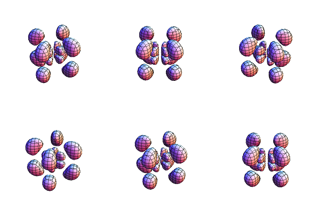
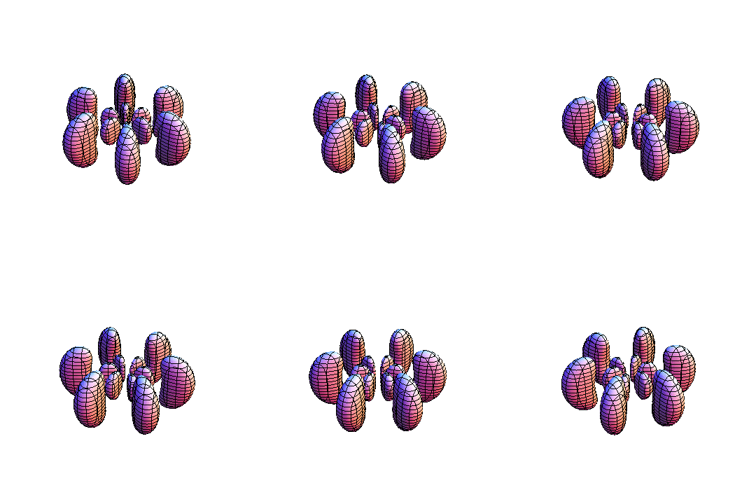
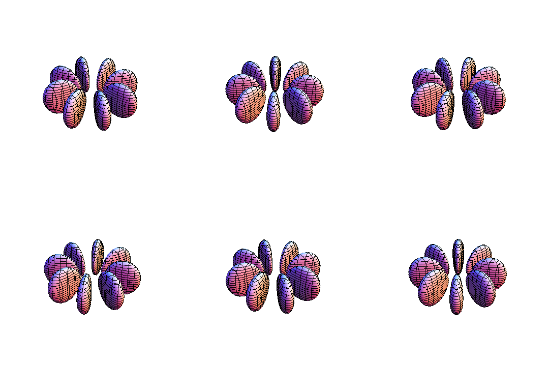
Download the original Mathematica notebook ↓ · Original hydrogen-state page ↗
Counting fringes, finding wavelengths.
The lab’s custom wavemeter compared an unknown laser with a reference using a scanning Michelson interferometer. My work included electronics fixes, calibration, control-software changes, and a manual documenting the instrument.
For the same change in optical path, fringe count is inversely proportional to wavelength. The reconstruction below follows the ratio in the 2013 manual:
λtest = λreference × Nreference / Ntest
Test wavelength:
Illustrative fringe-ratio calculation. It does not apply refractive-index corrections or estimate measurement uncertainty.
Read the preserved wavemeter manual ↗
Modeling the magnetic field.
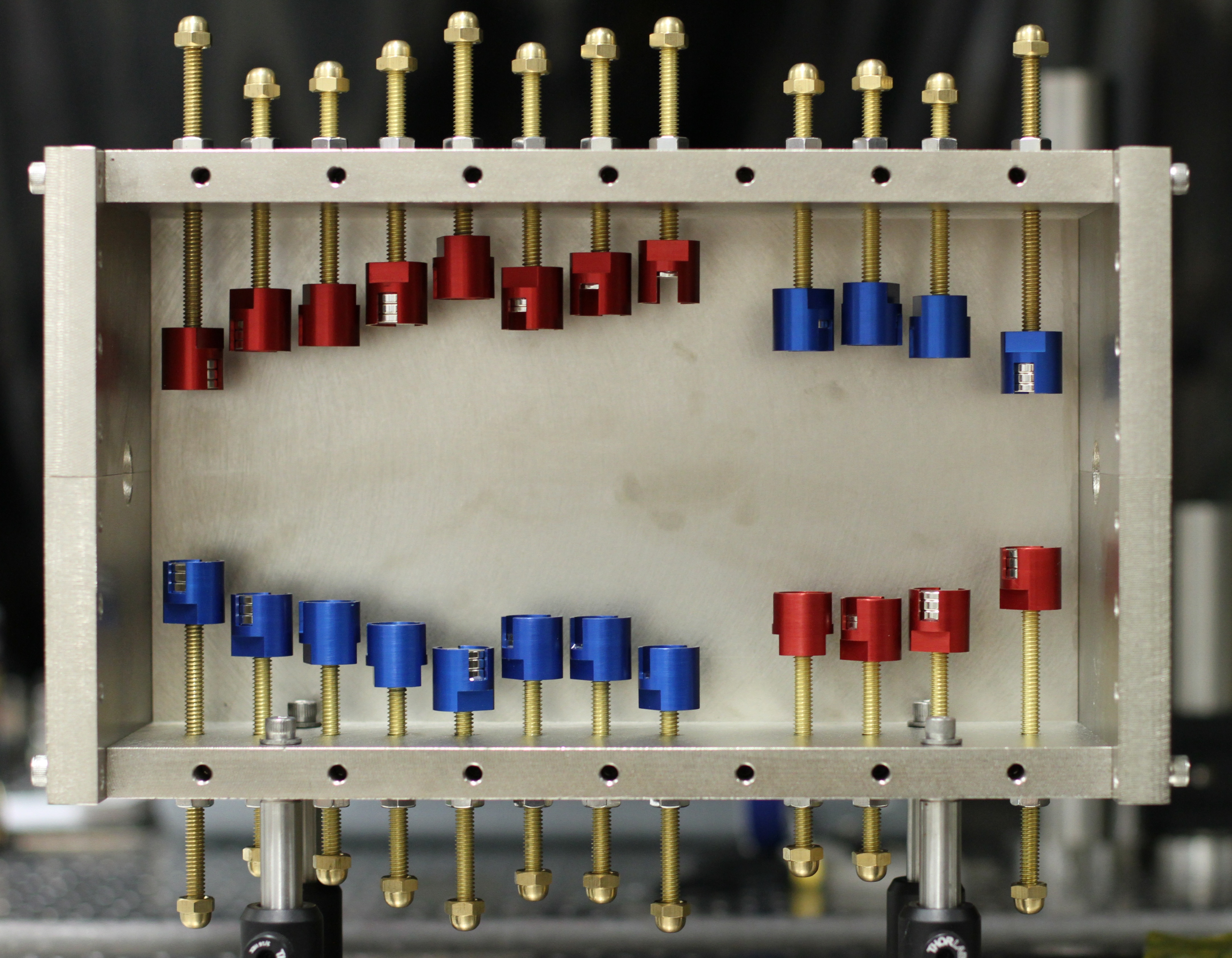
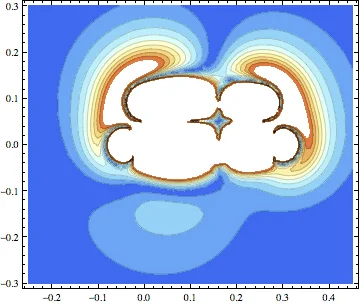
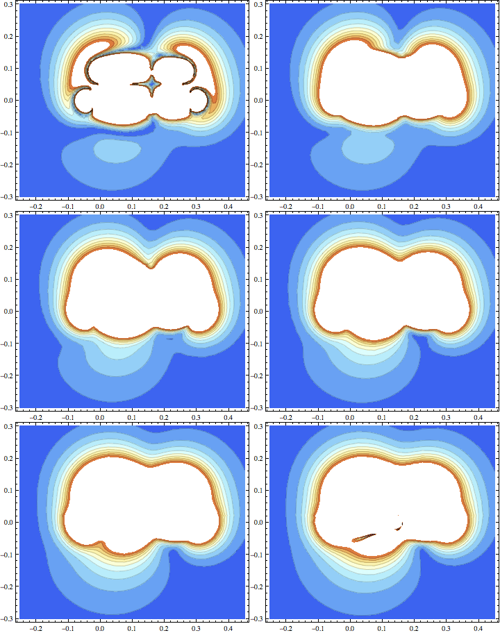
I used Mathematica to model magnetic dipoles and their images in the Zeeman slower’s housing. The original field animation explores the effect of removing a housing sidewall. The notebook and visualization are preserved below.
The original files.
Manuals, notebooks, and drawings from the public lab webpage. These are historical project files, preserved in their original formats.
-
Wavemeter user manual
2013 · PDF · 13 pages
-
Unibody Littrow laser notes
Original short write-up · PDF
-
Hydrogen-state visualizations
Original Mathematica notebook
-
Zeeman slower field model
Original Mathematica notebook
-
Driven harmonic motion
Original Mathematica notebook
-
Wavemeter alignment drawing
Original Vectorworks drawing
-
Fiber-couple mount
Original Vectorworks drawing
Retrieved September 6, 2026, from the original resource directory. The notebooks and CAD drawings download as files; they are not executed by this website.